Data Retrieval: IOER Monitor#
Summary
In this section, we will retrieve and visualize spatial data from the IOER Monitor.
In this section, we retrieve spatial data from the IOER Monitor using the Web Coverage Service (WCS). Specifically, we will access the indicator “Percentage of built-up settlement area and transport space to reference area” (Anteil baulich geprägter Siedlungs- und Verkehrsfläche an Gebietsfläche). This indicator describes the proportion of built-up settlement and transport space in an administrative territory and correlates with soil sealing and open space availability (IOER Monitor 2025).
The IOER Monitor data can be previewed in the geo viewer. The necessary WFS and WCS URLs, along with the unique indicator code (S12RG), can be found under Export → OGC Services.

Fig. 6 Densification of the block development in Berlin Friedrichshain. Photo: Jürgen Hohmuth, aus der Reihe “Gestalt des Raumes” (Buch und Ausstellung), © IOER-Media.#
IOER Monitor of Settlement and Open Space Development#
The IOER Monitor of Settlement and Open Space Development (short IOER Monitor) is a research data infrastructure provided by the Leibniz Institute of Ecological Urban and Regional Development (IOER). It offers insights into land use structure, development, and landscape quality in Germany. Indicators and data can be explored and visualized in an interactive geo viewer. All IOER Monitor data is available through Web Feature Service (WFS) and Web Coverage Service (WCS), allowing users to retrieve spatial data in standardized formats.
There are two ways to access and download data:
Via web browser: Login, search and download individual data files directly from the IOER Monitor’s download services.
Via code: Use the Monitor API to access data programmatically.
In both cases, registration is required.
Using the Monitor API
If you want to use the Monitor API, you need to register:
Register at monitor.ioer.de/monitor_api/signup.
Generate a personal API key in your account settings.
Store your personal API key in a file called
.envasAPI_KEY=xyz
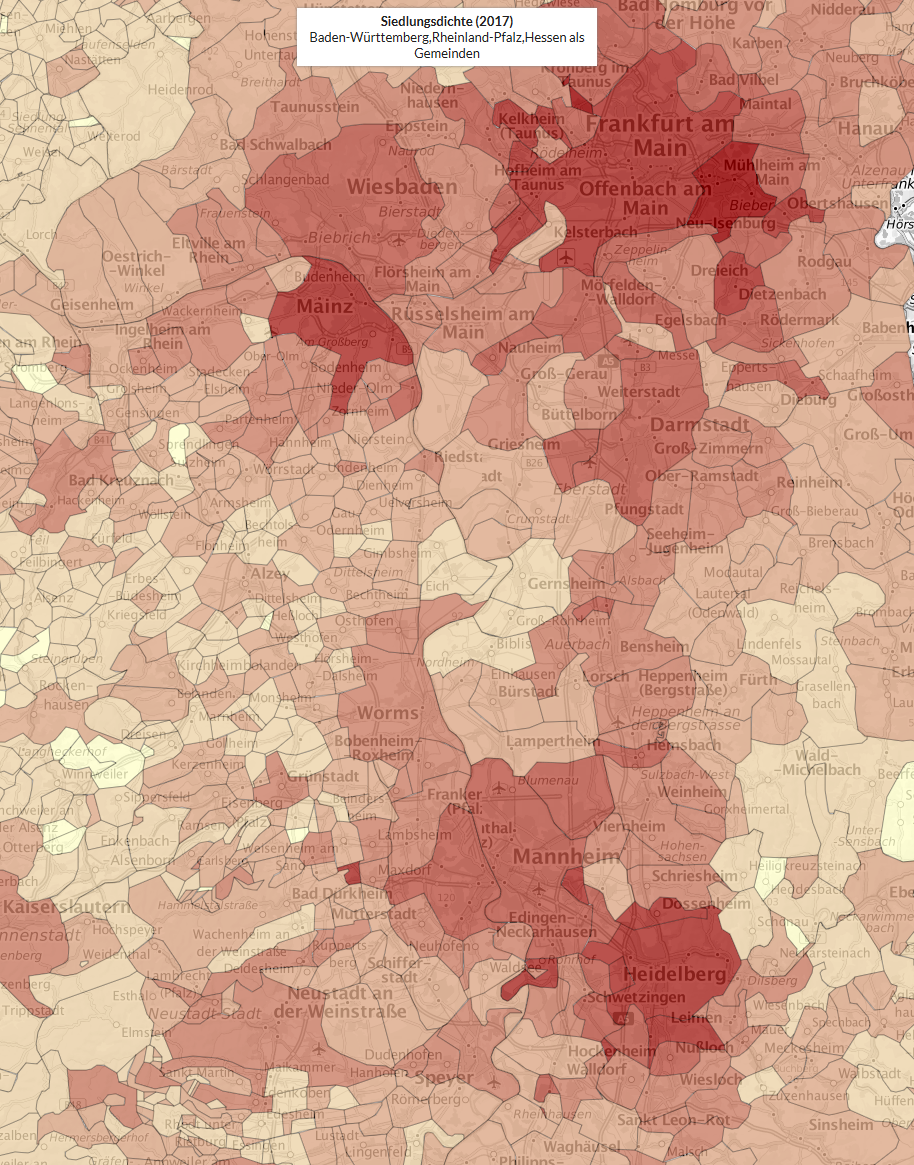
Fig. 7 Wie dicht leben wir? IOER Monitor data.#
Accessing IOER Monitor Data#
The IOER Monitor allows querying:
Raster data via Web Coverage Service (WCS)
Vector data via Web Feature Service (WFS)
To use the API programmatically, you need a personal API key. If you don’t have one yet, refer to the previous section for instructions.
Retrieving IOER Monitor API in Python#
Load dependencies
Before running the workflow, ensure the necessary libraries are installed and imported:
Show code cell source
# Standard library imports
import json
import os
import sys
import io
from pathlib import Path
from urllib.parse import urlencode

# Third-party imports
import matplotlib.pyplot as plt
import pandas as pd
import geopandas as gp
from IPython.display import display, Markdown
import rasterio
from rasterio.plot import show
from rasterio.mask import mask
from owslib.wcs import WebCoverageService
from lxml import etree
Load additional tools module
Show code cell source
base_path = Path.cwd().parent
module_path = str(base_path / "py")
if module_path not in sys.path:
    sys.path.append(module_path)
from modules import tools
Define parameters
To access the IOER Monitor data, we define two key parameters:
MONITOR_WCS_BASE: IOER Monitor API base endpointIOERMONITOR_WCS_ID: unique indicator code
MONITOR_WCS_BASE = "https://monitor.ioer.de/monitor_api/user" # API base endpoint
IOERMONITOR_WCS_ID = "S12RG" # Unique indicator code
Define the base path to store output files in this notebook
base_path = Path.cwd().parents[0]
OUTPUT = base_path / "out"
Secure API Key
To store your API key securely, use a dotenv (.env) file. This helps keep sensitive data safe and prevents accidental exposure:
Alternatively, use getpass()
If you don’t want to use an .env file, leave this step and you will be asked to directly enter the password in Jupyter below, by using getpass.getpass().
Create a file named
.envin the project root. Typically,.envfiles are added to.gitignorefiles to prevent them from being tracked.Add the following line:
IOERMONITOR_API_KEY=REPLACE-WITH-YOUR-PASSWORD # replace with your password
Load the key in your script:
from dotenv import load_dotenv
load_dotenv(
    Path.cwd().parents[0] / '.env', override=True)

MONITOR_API_KEY = os.getenv('IOERMONITOR_API_KEY')
You can continue without IOER Monitor Key
See Notebook 201 to register your IOER Monitor key. You can continue without an IOER Monitor API key, in which case you will only be able to view cached results below (e.g. for reproduction). If you want to retrieve new data (another region, etc.), register for a trial IOER Monitor key.
if MONITOR_API_KEY is None:
    import getpass
    MONITOR_API_KEY = getpass.getpass("Please enter your IOER Monitor API key")
    if not MONITOR_API_KEY:
        # user response empty
        print("Monitor API key not provided. Continuing with cached results..")
Querying WCS Data#
Configure API request
In order to connect to WCS services from Python, we use owslib (see documentation of owslib.wcs).
from urllib.parse import urlencode

params = {
    "id": IOERMONITOR_WCS_ID,
    "key": MONITOR_API_KEY,
    "service": "wcs",
}
wcs_url = f"{MONITOR_WCS_BASE}?{urlencode(params)}"

wcs = WebCoverageService(wcs_url, version="1.0.0") # WCS version `1.0.0`
Tip
When making requests to web APIs, you often need to pass parameters in a URL. However, some characters (such as spaces, special symbols, or non-ASCII characters) can cause issues if they are not properly encoded. urlencode prevents character encoding issues and improves readability. For more information, see urllib.parse module documentation
Explore Available Data
Let’s first run some checks on the returned wcs object and see what data we can access. The data is available for different time intervals and resolutions, as you can see below.
pd.DataFrame(wcs.contents.keys())
Show code cell output
| 0 | |
|---|---|
| 0 | S12RG_2000_100m |
| 1 | S12RG_2000_200m |
| 2 | S12RG_2000_500m |
| 3 | S12RG_2000_1000m |
| 4 | S12RG_2000_5000m |
| ... | ... |
| 109 | S12RG_2024_200m |
| 110 | S12RG_2024_500m |
| 111 | S12RG_2024_1000m |
| 112 | S12RG_2024_5000m |
| 113 | S12RG_2024_10000m |
114 rows × 1 columns
Select the dataset for 2023 at 200m raster resolution, which leads us to the key S12RG_2023_200m.
LAYER = 'S12RG_2023_200m'
Check the supported output formats for this layer.
if MONITOR_API_KEY: print(wcs.contents[LAYER].supportedFormats)
We can also query all additional available metadata for the layer (see dropdown below).
Show code cell source
layer_metadata = wcs.contents[LAYER]

print("Available Attributes for the Layer:")
if not MONITOR_API_KEY:
    print("Skipping because API key is not available.")
else:
    for attr in dir(layer_metadata):
        if not attr.startswith("_"):
            try:
                value = getattr(layer_metadata, attr)
                if attr == "descCov":
                    xml_content = etree.tostring(
                        value, pretty_print=True, encoding="unicode")
                    print(f"{attr} (XML Content):\n{xml_content}")
                else:
                    print(f"{attr}: {value}")
            except Exception as e:
                print(f"{attr}: Error accessing attribute - {e}")
Show code cell output
Available Attributes for the Layer:
Skipping because API key is not available.
Check the maximum available boundary for this layer. We can see that the limits are available in two different projections. In the following we will use the projected version of the boundary and not the WGS1984 version.
if MONITOR_API_KEY: print(wcs.contents[LAYER].boundingboxes)
Check the coordinate reference system (CRS).
if MONITOR_API_KEY: print(wcs.contents[LAYER].supportedCRS) # ['EPSG:3035']
Retrieve and visualize data
Set up query parameters and request the dataset.
BBOX = None
if MONITOR_API_KEY: BBOX = wcs.contents[LAYER].boundingboxes[1]["bbox"]
CRS = "EPSG:3035"
monitor_param = {
    "identifier": LAYER,
    "bbox": BBOX,
    "resx": 500,
    "resy": 500,
    "crs": CRS,
    "format": "GTiff"
}
if MONITOR_API_KEY: response = wcs.getCoverage(**monitor_param)
monitor_param
{'identifier': 'S12RG_2023_200m',
 'bbox': None,
 'resx': 500,
 'resy': 500,
 'crs': 'EPSG:3035',
 'format': 'GTiff'}
Load and display the GeoTiff with rasterio. If a cache exist, we prefer to load it directly (instead of querying the API again). If it does not exist, write it.
cache_file = OUTPUT / f"{LAYER}_DE.tiff"

if not cache_file.exists():
    if not MONITOR_API_KEY:
        if not Path(OUTPUT / "S12RG_2023_200m_DE.zip").exists():
            tools.get_zip_extract(
                output_path=OUTPUT,
                uri_filename="https://datashare.tu-dresden.de/s/HjGzHT7c3j36tai/download")
    else:
        # write to cache
        with open(cache_file, "wb") as f:
            f.write(response.read())
Loaded 4.17 MB of 4.18 (100%)..
Extracting zip..
Retrieved download, extracted size: 4.47 MB
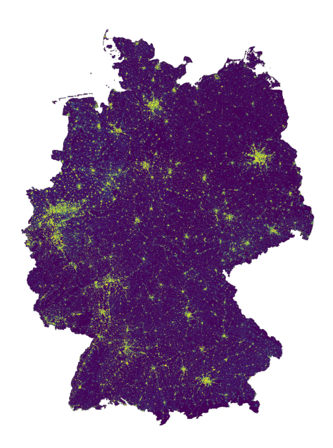
Visualize response (or cache).
with rasterio.open(cache_file) as src:
    fig, ax = plt.subplots(figsize=(8, 8))
    show(src, ax=ax)
    ax.axis('off')
Filtering data for Saxony#
However, we want to restrict the raster data to the following boundaries of the state of Saxony, similar to the way we restricted the responses for the GBIF Occurrence API.
Reproject the Saxony boundary to
EPSG:3035.Get boundaries (see section Data Retrieval: GBIF & LAND)
Update the monitor parameters (a Python dictionary) with the new
bbox.Get the grid with the new
bboxboundary
Restricting to Saxony boundaries
Load Saxony boundaries and reproject to match WCS layer.
sachsen_proj = gp.read_file(OUTPUT / 'saxony.gpkg')
BBOX = sachsen_proj.bounds.values.squeeze()
monitor_param["bbox"] = list(map(str, BBOX))
Retrieve and visualize clipped data using rasterio.show().
Check and retrieve cache
cache_file = OUTPUT / f"{LAYER}_Saxony.tiff"

if not cache_file.exists():
    if not MONITOR_API_KEY:
        if not Path(OUTPUT / "S12RG_2023_200m_Saxony.zip").exists():
            tools.get_zip_extract(
                output_path=OUTPUT,
                uri_filename="https://datashare.tu-dresden.de/s/Bm74ix6BDQtDzmP/download")
    else:
        # retrieve and write to cache
        response = wcs.getCoverage(**monitor_param)
        with open(cache_file, "wb") as f:
            f.write(response.read())
Loaded 0.28 MB of 0.28 (98%)..
Extracting zip..
Retrieved download, extracted size: 4.75 MB
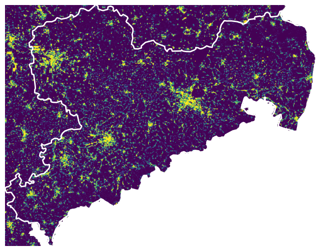
Visualize
with rasterio.open(cache_file) as src:
    fig, ax = plt.subplots(figsize=(8, 8))
    show(src, ax=ax)
    sachsen_proj.boundary.plot(
        ax=ax, color='white', linewidth=2)
    ax.axis('off')
Clipping the raster
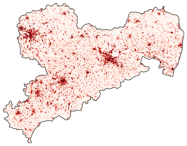
Use rasterio.mask to clip the raster with the boundaries of sachsen_proj. In addition, the cmap (a Matplotlib Colormap) is changed to Reds.
with rasterio.open(cache_file) as src:
    out_image, out_transform = mask(
        src, sachsen_proj.geometry, crop=True, filled=False)
    out_meta = src.meta.copy()
    fig, ax = plt.subplots(
        figsize=(8, 8))
    show(
        out_image,
        transform=out_transform,
        ax=ax, cmap='Reds')
    sachsen_proj.boundary.plot(
        ax=ax, color='black', linewidth=1)
    ax.axis('off')
See also
For a better understanding of the code, see the rasterio documentation.
Save the results to disk as a GeoTIFF. To do this, we first update the clipped raster meta object (out_meta) with the transformation information.
out_meta.update({
    "driver": "GTiff",
    "height": out_image.shape[1],
    "width": out_image.shape[2],
    "transform": out_transform,
    })
Then use rasterio.open() to write the clipped raster.
gtiff_path = OUTPUT / f'saxony_{LAYER}.tif'

with rasterio.open(gtiff_path, "w", **out_meta) as dest:
    dest.write(out_image)

# Get the file size in MB
file_size = gtiff_path.stat().st_size / (1024 * 1024)

print(f"GeoTIFF saved successfully. File size: {file_size:.2f} MB.")
GeoTIFF saved successfully. File size: 0.57 MB.
List of package versions used in this notebook
| package | python | geopandas | matplotlib | pandas | rasterio | requests | OWSLib |
|---|---|---|---|---|---|---|---|
| version | 3.12.13 | 1.1.3 | 3.10.9 | 2.3.3 | 1.5.0 | 2.34.2 | 0.35.0 |