From Footprints to Building Stock Insights

From Footprints to Building Stock Insights#

Authors: Markus Münzinger & Martin Behnisch (IOER)
Badges:

Background#

This notebook presents the core analysis from the Jupyter Book “From Footprints to Building Stock Insights” – a spatial decision-support pipeline for sustainable transformation. The work transforms 57 million building footprints across Germany into comparable building stock characteristics for evidence-based decision-making.

The Problem#

Germany has ~57 million buildings and structures, but this data is difficult to use directly:

Too many footprints to analyse individually
Complex 3D formats requiring specialised software
Large file sizes (~5 GB for the full dataset)
No direct comparability across municipalities

The Solution Pipeline#

The original book builds a pipeline that:

Assigns each footprint to its municipality (spatial join)
Aggregates data to administrative units
Combines with the RegioStaR spatial typology
Analyses the distribution of building stock
Visualises results for decision-makers

Dataset Used#

Name: 3D Building Metrics Germany 2024
DOI: 10.71830/9CBBWV
Source: Official 3D building models (LoD2)
Coverage: Germany (16 federal states), year 2024
Format: GeoParquet (~5 GB total)
License: CC BY 4.0

Book Structure (Original Chapters)#

Part	Chapters	Content
I	1–3	The dataset and the research question
II	4–5	Analytical highlights (Lorenz curves, Gini coefficients, maps)
III	6–7	From footprints to administrative data (full pipeline)
IV	8	Why the full pipeline is documented
V	9	Accessing the full dataset
VI	10	Reuse and adaptation

Key Finding (Preview)#

Metropolitan urban regions show the highest concentration of building volume (Gini = 0.669; top 10% of VWGs hold 60.3% of volume), compared to rural regions (Gini ≈ 0.42–0.44; top 10% ≈ 31–32%).

Applications#

Circular Economy: Identify regions with high building volume for material recycling potential
Energy Transition: Prioritise areas for energy-efficient retrofits
Urban Resilience: Understand building stock distribution for vulnerability and densification planning

This notebook focuses on the main analysis and results. For the full pipeline, data processing details, and reproduction steps, please refer to the complete Jupyter Book.

Chapter 5: Analysing Building Footprint Distributions#

Goal: Understand how building volume is distributed across VWGs within each RegioStaR4 class.

In this chapter, we:

Compute Lorenz curves for each RegioStaR4 class
Calculate Gini coefficients
Identify top 10% VWGs
Visualise results on maps

Note: This chapter uses the analytical dataset from Chapter 4 – no need for the full footprint dataset.

Setup#

First, let’s load the analytical dataset we created in Chapter 4.

# ============================================================
# Setup and load data
# ============================================================
from pathlib import Path
import pandas as pd
import geopandas as gpd
import numpy as np
import matplotlib.pyplot as plt
from matplotlib.colors import to_rgba
from matplotlib.patches import Patch

# Define root directory (two levels up from book/chapters/)
ROOT = Path.cwd().parent.parent

# Load the analytical dataset from Chapter 4 (CSV)
DATA_PATH = ROOT / "data" / "processed" / "vwg_building_stats_regiostar4.csv"
vwg_agg = pd.read_csv(
    DATA_PATH,
    dtype={
        'ars_vwg': 'object',
        'n_municipalities': 'int',
        'n_buildings': 'int',
        'total_volume_m3': 'float',
        'total_footprint_m2': 'float',
        'population': 'int',
        'vwg_name': 'object',
        'regiostar4_code': 'object',
        'regiostar4_name': 'object'
    }
)

# Path to VWG geometries
VG25_GPKG_PATH = ROOT / "data" / "raw" / "VG25" / "Daten" / "DE_VG25.gpkg"

print(f"Loaded {len(vwg_agg):,} VWGs")
print(f"Columns: {list(vwg_agg.columns)}")
print(f"VG25 file exists: {VG25_GPKG_PATH.exists()}")

Loaded 4,559 VWGs
Columns: ['ars_vwg', 'n_municipalities', 'n_buildings', 'total_volume_m3', 'total_footprint_m2', 'population', 'vwg_name', 'regiostar4_code', 'regiostar4_name']
VG25 file exists: True

What is a Lorenz Curve?#

A Lorenz curve shows how a resource (here: building volume) is distributed across a population (here: VWGs).

X-axis: Cumulative share of VWGs (sorted by volume, smallest to largest)
Y-axis: Cumulative share of building volume
Diagonal line: Perfect equality (every VWG has the same volume)

The further the curve bows below the diagonal, the more concentrated the volume is among a few VWGs.

What is the Gini Coefficient?#

A number between 0 and 1:

0 = perfect equality (all VWGs have the same volume)
1 = perfect inequality (one VWG has everything)

Lorenz Curve Function#

Let’s define a function to compute Lorenz curves and Gini coefficients.

# ============================================================
# Lorenz curve function
# ============================================================
def lorenz_curve(values):
    """
    Compute the Lorenz curve and Gini coefficient.
    
    Parameters:
        values: array-like of positive numbers
    
    Returns:
        cum_share_n: cumulative share of entities (x-axis)
        cum_share_value: cumulative share of values (y-axis)
        gini: Gini coefficient (0 = equal, 1 = concentrated)
    """
    # Sort values ascending
    values = np.sort(np.asarray(values, dtype=float))
    values = values[values >= 0]
    n = len(values)
    
    # Handle edge case
    if n == 0 or values.sum() == 0:
        return np.array([0, 1]), np.array([0, 1]), np.nan
    
    # Compute cumulative shares
    cum_values = np.cumsum(values)
    cum_share_value = np.insert(cum_values / cum_values[-1], 0, 0)
    cum_share_n = np.insert(np.arange(1, n + 1) / n, 0, 0)
    
    # Gini coefficient
    gini = 1 - 2 * np.trapezoid(cum_share_value, cum_share_n)
    
    return cum_share_n, cum_share_value, gini

Plot Lorenz Curves#

Let’s plot the Lorenz curves for each RegioStaR4 class.

How to read this chart:

X-axis: Cumulative share of VWGs (sorted by volume, smallest to largest)
Y-axis: Cumulative share of building volume
Diagonal line: Perfect equality (every VWG has the same volume)

What to look for:

Closer to the diagonal – More equal distribution
Further from the diagonal – More concentrated distribution (a few VWGs hold most of the volume)

# ============================================================
# Plot Lorenz curves by RegioStaR4
# ============================================================
# Labels for RegioStaR4 classes
regiostar4_labels = {
    '11': 'Metropolitan urban',
    '12': 'Regiopolitan urban',
    '21': 'Rural close to urban',
    '22': 'Peripheral rural'
}

# Create plot
fig, ax = plt.subplots(figsize=(8, 8))

# Perfect equality line
ax.plot([0, 1], [0, 1], 'k--', label='Perfect equality', linewidth=1)

# Plot each class
for code in ['11', '12', '21', '22']:
    group = vwg_agg[vwg_agg['regiostar4_code'] == code]
    x, y, gini = lorenz_curve(group['total_volume_m3'])
    label = f"{regiostar4_labels[code]} (Gini={gini:.3f}, n={len(group)})"
    ax.plot(x, y, label=label, linewidth=2)

ax.set_xlabel('Cumulative share of VWGs', fontsize=12)
ax.set_ylabel('Cumulative share of building volume', fontsize=12)
ax.set_title('Concentration of Building Volume by RegioStaR4', fontsize=14)
ax.legend(loc='lower right', fontsize=10)
ax.grid(True, alpha=0.3)
plt.tight_layout()
plt.show()

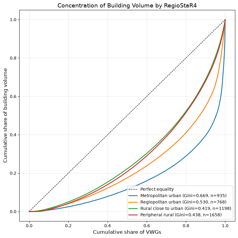
../_images/4ec03dd0e638c4cd1e91b9e312df95dba1682386d8959ecd2a4529439a7133c7.png

What the Curves Show#

Metropolitan urban (red) – Curve bows furthest from the diagonal → highest concentration
Regiopolitan urban (blue) – Moderate bow → noticeable concentration
Rural close to urban (green) – Closest to diagonal → lowest concentration, but still moderate
Peripheral rural (purple) – Similar to green → moderate concentration

All classes show moderate to high concentration – none are close to perfect equality.

Concentration Metrics#

To quantify these patterns, we compute:

Gini coefficient – 0 = perfect equality, 1 = perfect concentration
Top 10% share – What percentage of total building volume is held by the largest 10% of VWGs in each class
Top 20% share – What percentage of total building volume is held by the largest 20% of VWGs in each class

Why these metrics matter:

Gini – Summarises overall inequality in one number
Top 10%/20% shares – Show how much volume is controlled by the largest VWGs – useful for identifying dominant centers

# ============================================================
# Concentration metrics by RegioStaR4
# ============================================================
print(f"{'Class':<25} {'VWGs':>6} {'Gini':>8} {'Top10% VWGs':>12} {'Top20% VWGs':>12}")
print("-" * 65)

for code in ['11', '12', '21', '22']:
    group = vwg_agg[vwg_agg['regiostar4_code'] == code]
    
    # Compute Gini
    x, y, gini = lorenz_curve(group['total_volume_m3'])
    
    # Sort volumes descending
    sorted_vals = np.sort(group['total_volume_m3'].values)[::-1]
    total_vol = sorted_vals.sum()
    
    # Top 10% share
    n_top10 = max(1, int(len(group) * 0.1))
    top10_share = sorted_vals[:n_top10].sum() / total_vol * 100
    
    # Top 20% share
    n_top20 = max(1, int(len(group) * 0.2))
    top20_share = sorted_vals[:n_top20].sum() / total_vol * 100
    
    print(f"{regiostar4_labels[code]:<25} {len(group):>6,} {gini:>8.3f} {top10_share:>11.1f}% {top20_share:>11.1f}%")

Class                       VWGs     Gini  Top10% VWGs  Top20% VWGs
-----------------------------------------------------------------
Metropolitan urban           935    0.669        60.3%        71.1%
Regiopolitan urban           768    0.530        45.0%        58.9%
Rural close to urban       1,198    0.419        31.0%        47.7%
Peripheral rural           1,658    0.438        31.9%        48.4%

Interpretation#

Metropolitan urban (Gini = 0.669): Highest concentration. Top 10% of VWGs hold 60% of building volume.
Regiopolitan urban (Gini = 0.530): Moderate concentration.
Rural close to urban (Gini = 0.419): More equal distribution.
Peripheral rural (Gini = 0.438): Similar to rural close to urban.

Key insight: Building volume is most concentrated in metropolitan areas – a few large cities dominate.

Why Split by RegioStaR4?#

Before looking at the maps, let’s examine the actual building volumes per class.

Why this matters:

Without splitting by RegioStaR4, the analysis would be dominated by metropolitan urban regions – they have the highest volume per VWG and the highest concentration (Gini = 0.669).

By splitting into classes, we can:

Compare structurally similar municipalities
Identify patterns within each region type
Avoid the analysis being skewed by a few large cities

# ============================================================
# Building volume by RegioStaR4 class
# ============================================================
volume_by_class = vwg_agg.groupby(['regiostar4_code', 'regiostar4_name']).agg(
    n_vwgs=('ars_vwg', 'count'),
    total_volume_m3=('total_volume_m3', 'sum')
).reset_index()

# Calculate share of total volume
total_volume_all = volume_by_class['total_volume_m3'].sum()
volume_by_class['share_of_total'] = volume_by_class['total_volume_m3'] / total_volume_all * 100

# Calculate volume per VWG
volume_by_class['volume_per_vwg'] = volume_by_class['total_volume_m3'] / volume_by_class['n_vwgs']

# Format for display
display_df = volume_by_class.copy()
display_df['total_volume_m3'] = display_df['total_volume_m3'].map(lambda x: f"{x/1e9:.1f} billion")
display_df['share_of_total'] = display_df['share_of_total'].map(lambda x: f"{x:.1f}%")
display_df['volume_per_vwg'] = display_df['volume_per_vwg'].map(lambda x: f"{x/1e6:.1f} million m³")

display_df.columns = ['Code', 'Class', 'VWGs', 'Total Volume', 'Share of Total', 'Volume per VWG']
print("Building volume by RegioStaR4 class:")
display(display_df)

Building volume by RegioStaR4 class:

	Code	Class	VWGs	Total Volume	Share of Total	Volume per VWG
0	11	Metropolitan urban region	935	16.4 billion	34.9%	17.6 million m³
1	12	Regiopolitan urban region	768	9.3 billion	19.9%	12.1 million m³
2	21	Rural region close to an urban region	1198	10.3 billion	21.9%	8.6 million m³
3	22	Peripheral rural region	1658	10.9 billion	23.3%	6.6 million m³

What the Table Shows#

RegioStaR4	VWGs	Total Volume	Share	Volume per VWG
Metropolitan urban	935	16.4 billion m³	34.9%	17.6 million m³
Regiopolitan urban	768	9.3 billion m³	19.9%	12.1 million m³
Rural close to urban	1,198	10.3 billion m³	21.9%	8.6 million m³
Peripheral rural	1,658	10.9 billion m³	23.3%	6.6 million m³

Key observations:

Metropolitan urban – Highest volume per VWG (17.6 million m³) – large cities dominate
Peripheral rural – Most VWGs (1,658) but lowest volume per VWG (6.6 million m³)
Rural areas combined hold about 45% of total building volume – a substantial share

This confirms why splitting by RegioStaR4 is useful – without it, the analysis would be dominated by metropolitan regions.

Identify Top 10% VWGs#

Let’s identify which VWGs belong to the top 10% in each class.

This step prepares the data for the maps later in this chapter – we’ll highlight these top VWGs visually to see where the largest building volumes are concentrated across Germany.

# ============================================================
# Identify top 10% VWGs per RegioStaR4 class
# ============================================================
top10_vwgs = []

for code in ['11', '12', '21', '22']:
    group = vwg_agg[vwg_agg['regiostar4_code'] == code].copy()
    group = group.sort_values('total_volume_m3', ascending=False)
    n_top10 = max(1, int(len(group) * 0.1))
    group['top10'] = False
    group.iloc[:n_top10, group.columns.get_loc('top10')] = True
    top10_vwgs.append(group[['ars_vwg', 'regiostar4_code', 'regiostar4_name', 
                              'total_volume_m3', 'top10']])

top10_df = pd.concat(top10_vwgs, ignore_index=True)
print(f"Identified top 10% VWGs: {top10_df['top10'].sum():,}")
top10_df[top10_df['top10'] == True].head(10)

Identified top 10% VWGs: 453

	ars_vwg	regiostar4_code	regiostar4_name	total_volume_m3	top10
0	110000000	11	Metropolitan urban region	1.263238e+09	True
1	020000000	11	Metropolitan urban region	7.320077e+08	True
2	091620000	11	Metropolitan urban region	4.972838e+08	True
3	053150000	11	Metropolitan urban region	4.234902e+08	True
4	064120000	11	Metropolitan urban region	3.374048e+08	True
5	040110000	11	Metropolitan urban region	2.941626e+08	True
6	051110000	11	Metropolitan urban region	2.775604e+08	True
7	147130000	11	Metropolitan urban region	2.622065e+08	True
8	032410001	11	Metropolitan urban region	2.518303e+08	True
9	081110000	11	Metropolitan urban region	2.516939e+08	True

Load VWG Geometries#

Now let’s load the VWG polygons for mapping.

So far, we’ve worked with aggregated data on municipal associations (Gemeindeverbände) – derived from individual municipalities (Gemeinden).

For the map, we now join this data to the actual geometries of these associations. We load them from the VG25 GeoPackage (layer: vg25_vwg), which contains the official administrative boundaries provided by BKG.

# ============================================================
# Load VWG geometries
# ============================================================
print("Loading VWG geometries...")
vwg_geom = gpd.read_file(VG25_GPKG_PATH, layer='vg25_vwg', engine='pyogrio')
print(f"Loaded {len(vwg_geom):,} VWG polygons")

# Join top 10% data to geometries
vwg_geom_join = vwg_geom.merge(top10_df, left_on='ARS', right_on='ars_vwg', how='inner')
print(f"Joined: {len(vwg_geom_join):,} VWGs with geometry")

Loading VWG geometries...
Loaded 4,599 VWG polygons
Joined: 4,559 VWGs with geometry

Map: Top 10% VWGs by RegioStaR4 Class#

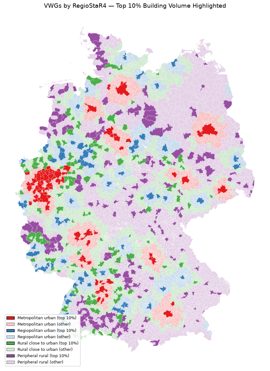
Now let’s visualise the top 10% VWGs on a map.

Why this map matters:

The analysis by RegioStaR4 enables us to see differentiated patterns across Germany – patterns that would otherwise be dominated by urban Gemeindeverbände.

By splitting into four classes and highlighting the top 10% within each, we can see:

Where the largest building volumes are concentrated within each region type
How the spatial patterns differ between metropolitan, regiopolitan, and rural areas
Which VWGs stand out – beyond just the big cities

Color scheme:

Red – Metropolitan urban regions
Blue – Regiopolitan urban regions
Green – Rural regions close to urban areas
Purple – Peripheral rural regions

Full color = top 10% VWGs (highlighted)
Faded color = other VWGs in that class

# ============================================================
# Single map with all classes
# ============================================================
# Color scheme for each RegioStaR4 class
class_colors = {
    '11': '#e41a1c',  # red
    '12': '#377eb8',  # blue
    '21': '#4daf4a',  # green
    '22': '#984ea3'   # purple
}

# Create color column
def get_color(row):
    base_color = to_rgba(class_colors[row['regiostar4_code']])
    if row['top10']:
        return base_color  # full saturation
    else:
        return (base_color[0], base_color[1], base_color[2], 0.25)  # faint

vwg_geom_join['color'] = vwg_geom_join.apply(get_color, axis=1)

# Plot
fig, ax = plt.subplots(figsize=(14, 12))

# Plot all VWGs
vwg_geom_join.plot(ax=ax, color=vwg_geom_join['color'], edgecolor='white', linewidth=0.2)

# Add legend
legend_elements = []
for code, color in class_colors.items():
    legend_elements.append(
        Patch(facecolor=color, edgecolor='black', label=f"{regiostar4_labels[code]} (top 10%)")
    )
    legend_elements.append(
        Patch(facecolor=to_rgba(color, alpha=0.25), edgecolor='grey', 
              label=f"{regiostar4_labels[code]} (other)")
    )

ax.legend(handles=legend_elements, loc='lower left', fontsize=9, framealpha=0.9)
ax.set_title('VWGs by RegioStaR4 — Top 10% Building Volume Highlighted', fontsize=14)
ax.axis('off')
plt.tight_layout()
plt.show()


# ============================================================
# Save the map for use in other chapters
# ============================================================
images_dir = ROOT / "images"
images_dir.mkdir(parents=True, exist_ok=True)
fig.savefig(images_dir / "map_top10_single.png", dpi=300, bbox_inches='tight')
print(f"Map saved to: {images_dir / 'map_top10_single.png'}")

../_images/9b7eae863bcd3f2489d4694649834c5fb3c574de1a0042a719512bf3f0db7fcb.png

Map saved to: A:\tarox03_user4\Muenzinger\8_current_processing\ioer_hacklathon_3d_building_metrics_2024\3d-building-pareto-analysis\images\map_top10_single.png

What This Means for Your Work#

The maps reveal distinct spatial patterns of building volume concentration across Germany:

Metropolitan regions – Volume is highly concentrated in a few large centers
Rural regions – Volume is more evenly distributed across many VWGs

These patterns are not just descriptive – they are actionable. We invite you to explore, adapt, and extend the pipeline to your own research questions – whether in the circular economy, energy transition, or urban resilience.

Try It Yourself#

Here are some ideas to get started:

Use roof area instead of building volume
Change the threshold – top 5% or top 20%
Compute Gini for roof area
Compare RegioStaR2 vs RegioStaR4

Modify the code above and see what patterns emerge!

Summary#