
From Footprints to Building Stock Insights#
Authors: Markus Münzinger & Martin Behnisch (IOER)
Badges:




The Research Challenge#
Germany’s built environment consists of approximately 57 million buildings and structures. While high-resolution 3D building models (LoD2) provide unprecedented detail, the sheer volume of data creates a significant barrier to evidence-based decision-making.
The challenge: transforming raw geospatial data (millions of individual polygons) into comparable building stock characteristics that can be analyzed across different administrative and spatial scales.
The Dataset: 3D Building Metrics Germany 2024#
This analysis leverages the 3D Building Metrics Germany 2024 dataset:
Münzinger, Markus, 2026, “3D Building Metrics Germany 2024”,
https://doi.org/10.71830/9CBBWV, ioerDATA, V1
Property |
Value |
|---|---|
Buildings & structures |
57,326,925 |
Source |
Official 3D building models (LoD2) |
Year |
2024 |
Coverage |
Germany (16 federal states) |
Format |
GeoParquet (one file per state) |
Total size |
~5 GB |
License |
|
Spatial base data |
© GeoBasis-DE / BKG (2025) – Terms of Use |
Each building footprint contains 14 attributes, including:
Column |
Description |
|---|---|
|
Building volume (m³) |
|
Roof area (m²) |
|
Wall area (m²) |
|
Footprint area (m²) |
|
Building function code |
|
Polygon geometry |
⚠️ Not everything is a building. The dataset includes bridges, silos, wind turbines, and sound barriers. Throughout this book, we filter to buildings only using function codes starting with
31.
The Building Stock Insights Pipeline#
To bridge the gap between raw data and meaningful analysis, we developed a Building Stock Insights Pipeline that transforms nationwide building footprints into aggregated metrics for comparative analysis.
The workflow follows five steps:
Large Geospatial Dataset → Spatial Assignment → Aggregation → Classification → Analysis
Large Geospatial Dataset: Accessing enriched 3D building metrics.
Spatial Assignment: Efficiently joining footprints to administrative boundaries.
Aggregation: Distilling individual metrics into municipal-level characteristics.
Classification: Integrating spatial typologies (e.g., RegioStaR) to categorize the urban-rural continuum.
Analysis: Applying statistical methods (e.g., Lorenz curves) to identify structural patterns.
Preview of Results#
The pipeline’s output reveals the concentration of building volume across Germany, differentiated by settlement typology:
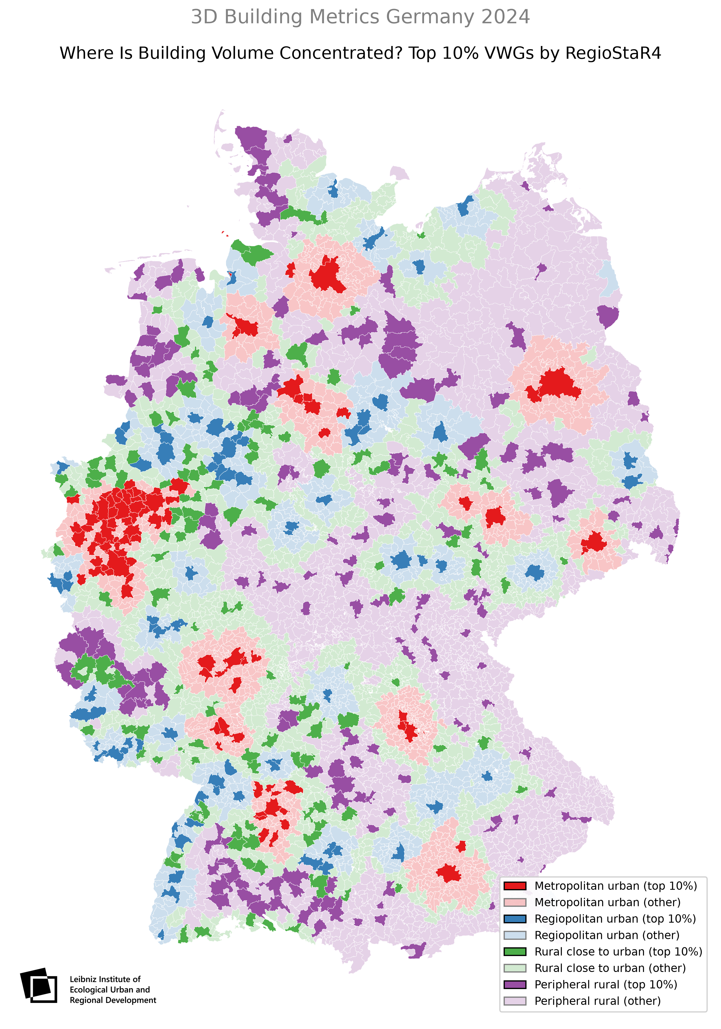
Fig. 12 Top 10% VWGs by building volume, colored by RegioStaR4 class. Spatial base data: © GeoBasis-DE / BKG (2025) .#
This map gives a first glimpse of the patterns we explore in the analysis subchapter. We’ll dive into the methods and interpretations together — but already visible are:
Where the largest building volumes are concentrated across Germany.
How patterns differ between metropolitan, regiopolitan, and rural regions.
Why splitting by RegioStaR4 reveals insights that would otherwise be dominated by urban areas.
The “So What?”: Connecting Data to Sustainability#
The value of this pipeline lies not in the aggregation itself, but in the insights it enables. By identifying how building volume and roof areas are distributed, we can address concrete sustainability challenges:
🏭 Circular Economy: Where are building materials concentrated? Identifying regions with high building volume to map material stocks and recycling potential.
⚡ Energy Transition: Where is renovation potential highest? Prioritizing regions for energy-efficient retrofits based on building stock characteristics.
🌆 Urban Resilience: How is building stock distributed across regions? Understanding vulnerability and planning for densification and climate adaptation.
Your challenge: The HaCLAthon invites you to explore, adapt, and extend this pipeline to address these — or your own — sustainability questions. We’re curious to see what patterns you uncover and how you connect them to real-world applications.
How to Use This Chapter#
This chapter is organized into three subchapters:
Subchapter |
Content |
Execution |
|---|---|---|
Hands-on exploration of the raw data (Saarland) |
✅ Runs |
|
Lorenz curves, Gini coefficients, spatial mapping, “Try It Yourself” adaptations |
✅ Runs |
|
Full spatial join and aggregation pipeline (DuckDB, 5 GB dataset) |
📄 Documentation only |
Subchapter 2 is your starting point for the HaCLAthon. It runs on provided data — no download needed. You can adapt the analysis to explore different metrics (e.g., roof area instead of volume) or different thresholds (e.g., top 5% instead of top 10%).
Subchapter 3 is documentation — not executed in this book. It shows how we processed the full 5 GB dataset using DuckDB and spatial joins. We document it for:
Reproducibility — best practice for open science
Showcasing — how to work with large GeoParquet datasets efficiently
Inspiration — a potential template for your own large-scale analyses
💡 For the HaCLAthon: Start with Subchapter 2. It gives you immediate results and a clear path to extend the analysis. Subchapter 3 is there if you want to go deeper into the data engineering side.
Citation#
If you use this dataset or the pipeline in your work, please cite:
@book{muenzinger2026footprints,
  title={From Footprints to Building Stock Insights},
  author={Münzinger, Markus and Behnisch, Martin},
  year={2026},
  publisher={IOER}
}

@dataset{muenzinger2026dataset,
  title={3D Building Metrics Germany 2024},
  author={Münzinger, Markus},
  year={2026},
  publisher={ioerDATA},
  doi={10.71830/9CBBWV}
}