1. The Data Up Close: Saarlouis

Before analyzing nationwide patterns, let’s understand the granularity of the source data. We use the area around Saarlouis — a historic town in southwestern Germany — as example. It is ideal for exploration without requiring high-performance computing.

Setup

First, we set up our environment and define paths to the data. Since we’re working with a pre-filtered subset (the Saarlouis bounding box), we can use GeoPandas to read the data directly into memory — no need for the heavy-duty processing tools required for the full 5 GB dataset.

# ============================================================
# Setup and paths
# ============================================================
from pathlib import Path
import geopandas as gpd
import pandas as pd
import matplotlib.pyplot as plt

# Define root directory (adjust if needed)
ROOT = Path.cwd().parent

# Path to Saarlouis bounding box partition
SAARLOUIS_PATH = ROOT / "data" / "raw" / "3D_building_metrics_germany_2024" / "saarlouis_bbox_3d_building_metrics_2024.parquet"

# Filter: only buildings (function code starts with '31')
BLDG_FUNCTION_PREFIX = "31"

print(f"Saarlouis file exists: {SAARLOUIS_PATH.exists()}")

Saarlouis file exists: True

💡 Why GeoPandas here? This subchapter works with a pre-filtered subset (~61,000 footprints) that fits comfortably in memory. GeoPandas provides a familiar, intuitive interface for exploration and visualization. For the full 5 GB dataset (3. Building the Analytical Foundation), we switch to DuckDB — an in-process analytical database that handles large spatial data efficiently with spatial indexes and parallel processing. The choice of tool depends on the data size and task at hand.

Load and Filter

Now we load the Saarlouis footprints and filter to buildings only. The dataset contains not only buildings but also structures like bridges, silos, and wind turbines — identified by their function codes.

# ============================================================
# Load Saarlouis footprints
# ============================================================
print("Loading Saarlouis footprints...")
saarlouis = gpd.read_parquet(SAARLOUIS_PATH)

print(f"Total footprints: {len(saarlouis):,}")
print(f"Columns: {list(saarlouis.columns)}")
print()

# Filter to buildings only
saarlouis_buildings = saarlouis[saarlouis['bldg_function'].str.startswith(BLDG_FUNCTION_PREFIX)].copy()
print(f"Buildings (function '31*'): {len(saarlouis_buildings):,}")
print(f"Excluded structures: {len(saarlouis) - len(saarlouis_buildings):,}")

Loading Saarlouis footprints...
Total footprints: 60,368
Columns: ['bldg_gmlid', 'count_bldg_parts', 'bldg_function', 'bldg_volume', 'bldg_max_measured_height', 'count_roof_surfaces', 'roof_area', 'count_wall_surfaces', 'wall_area', 'footprint_area', 'footprint_perimeter', 'geometry']

Buildings (function '31*'): 58,741
Excluded structures: 1,627

Visualize Footprints

Let’s look at the actual building footprints in the Saarlouis area to understand the spatial patterns and density of the building stock.

# ============================================================
# Plot footprints for the Saarlouis area
# ============================================================
fig, ax = plt.subplots(figsize=(12, 10))

# Plot footprints
saarlouis_buildings.plot(ax=ax, color='steelblue', edgecolor='white', linewidth=0.2)

ax.set_title(f"Building Footprints in Saarlouis Area ({len(saarlouis_buildings):,} buildings)")
ax.set_xlabel("Easting (m)")
ax.set_ylabel("Northing (m)")
ax.set_aspect('equal')
plt.tight_layout()
plt.show()

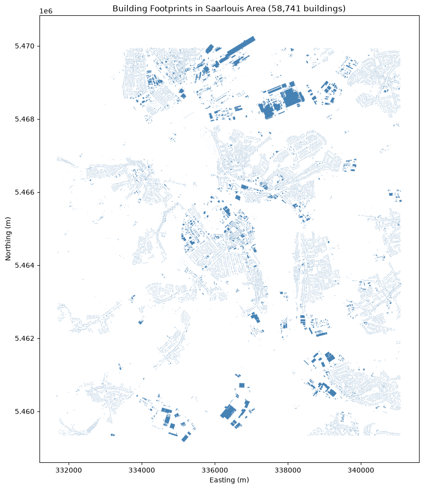
The map reveals distinct patterns in building size and density. We can see clusters of buildings with similar footprint sizes — small, densely packed structures in the historic core contrast with larger, more spread-out buildings in industrial and commercial areas. The varying building densities across the area reflect different urban development phases and land use types. The Saar river meanders through the region, creating natural boundaries that shape the urban form.

Basic Statistics

The visual impression of heterogeneous building sizes and densities can be quantified through summary statistics. Let’s compute key metrics to characterize the building stock in the Saarlouis area.

# ============================================================
# Summary statistics
# ============================================================
summary = saarlouis_buildings[['bldg_volume', 'footprint_area', 'roof_area', 'bldg_max_measured_height']].describe().T

# Format for readability
summary['count'] = summary['count'].astype(int).map(lambda x: f"{x:,}")
for col in ['mean', 'std', 'min', '25%', '50%', '75%', 'max']:
    summary[col] = summary[col].map(lambda x: f"{x:,.1f}")

# Rename columns for clarity
summary = summary.rename(columns={
    '25%': 'Q1 (25th)',
    '50%': 'Median (50th)',
    '75%': 'Q3 (75th)'
})

summary.index = ['Volume (m³)', 'Footprint (m²)', 'Roof area (m²)', 'Height (m)']
print("Summary statistics for Saarlouis buildings:")
display(summary)

Summary statistics for Saarlouis buildings:

	count	mean	std	min	Q1 (25th)	Median (50th)	Q3 (75th)	max
Volume (m³)	58,741	1,109.7	17,980.1	1.9	90.4	426.4	865.5	3,453,114.7
Footprint (m²)	58,741	129.5	1,209.5	1.4	27.1	66.3	113.0	161,507.5
Roof area (m²)	58,741	141.7	1,211.6	1.5	28.8	75.5	135.2	161,507.5
Height (m)	58,741	6.9	3.9	1.0	3.3	6.8	9.8	69.3

Key Insight: The mean is higher than the median for all metrics — a right-skewed distribution. Most buildings have comparable dimensions at the lower end of the scale, but a few large outliers (e.g., industrial halls, high-rise structures) are substantially larger than the average. This heterogeneity within the building stock is itself an important characteristic — it means that aggregated metrics need to be interpreted with care, as they may be strongly influenced by a small number of exceptional structures.

From Local Detail to Germany-Wide Patterns

We’ve now seen what the data looks like at the building level. But our goal is to understand Germany-wide patterns.

To do this, we need to:

1. Aggregate individual footprints to administrative units

2. Combine with spatial classifications (RegioStaR)

3. Analyze the distribution of building stock across all regions

This is exactly what we’ll do in 2. Analyzing Building Stock Patterns.